Mendelian Randomization: Using Genetics as Nature's Randomized Trial
You run a study showing that higher HDL cholesterol is associated with lower cardiovascular risk. But is it causal? You cannot randomize people to have different cholesterol levels. Nature, however, already did. Mendelian randomization (MR) exploits the fact that genetic variants are allocated randomly at conception — a biological lottery that creates something close to an RCT embedded in observational data.
In this guide
- 1. What Mendelian randomization is (and why it matters)
- 2. Three assumptions — translated for genetic data
- 3. Study design: one-sample vs. two-sample MR
- 4. Choosing genetic instruments: the modern pipeline
- 5. Pleiotropy: the central threat to MR validity
- 6. Estimation methods: from IVW to MR-PRESSO
- 7. Six ways MR studies fail
- 8. Reporting checklist for MR studies
- 9. Automated MR critique with Aqrab
1. What Mendelian randomization is (and why it matters)
Mendelian randomization uses genetic variants as instrumental variables to estimate the causal effect of an exposure on an outcome. The key insight is Mendel's second law of independent assortment: alleles are shuffled randomly during meiosis, meaning genetic variants are approximately independent of confounders that plague observational studies.
The biological randomization analogy
Think of it this way: nature randomly assigns people to have different levels of a biomarker (through their genotype). That random assignment at conception is what makes MR powerful. A person with alleles that produce higher LDL cholesterol from birth is, in a sense, "randomly assigned" to higher LDL — not because they chose a poor diet, but because their genes allocated them that way.
MR has exploded in popularity because of publicly available GWAS summary statistics. You no longer need individual-level genetic data — with two-sample MR, you can use published GWAS results for the exposure (e.g., a large UK Biobank study on BMI) and the outcome (e.g., a global consortium study on coronary artery disease) from separate datasets. This has made MR accessible to any researcher with a laptop and an internet connection. The problem: that accessibility has produced a flood of low-quality MR studies that violate assumptions in ways the authors don't understand.
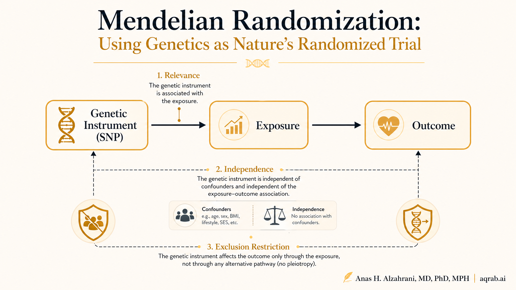
2. Three assumptions — translated for genetic data
MR inherits the instrumental variable assumptions, but the genetic context adds specific implications:
The SNPs must be associated with the exposure
Each genetic variant must meaningfully affect the exposure. With multiple SNPs, the F-statistic should exceed 10 (preferably much higher). In practice, this means selecting variants from large GWAS with strong, well-validated signals. Weak instrument bias in MR is the same as in 2SLS — biased toward the observational estimate and with artificially narrow confidence intervals.
The SNPs must not be associated with confounders
Population stratification is the primary threat. If your GWAS included people of different genetic ancestries, and ancestry correlates with both the exposure and the outcome through environmental or cultural pathways, your SNPs are not independent of confounders. This is partially addressable by restricting to a single ancestry group or using methods like MR-Egger that can detect some forms of directional pleiotropy.
The SNPs must affect the outcome only through the exposure
In MR, this assumption is called the no horizontal pleiotropy assumption. A SNP that raises HDL cholesterol but also independently affects inflammation (through a different biological pathway) violates the exclusion restriction. This is the most dangerous threat in MR because it is extremely common in biology — genes are networked, pleiotropic, and messy. It is also the assumption you can never fully test.
3. Study design: one-sample vs. two-sample MR
MR studies come in two main flavors, and the distinction matters enormously:
One-sample MR
Genotype data, exposure, and outcome all come from the same individuals. You regress the outcome on the genetic instrument using individual-level data. Classic 2SLS approach.
Pro: Directly testable
Can check instrument strength in your own sample. No sample overlap issues.
Con: Requires individual-level genetic data
Expensive, ethically complex, rarely feasible for meta-analyses.
Two-sample MR
Instrument-exposure associations come from one GWAS, instrument-outcome associations from a different GWAS. Estimates are computed from summary statistics alone — no individual data needed.
Pro: Vastly more accessible
Leverage GWAS summary statistics from thousands of publicly available studies.
Con: Inherent assumptions about sample equivalence
Two-sample MR is valid only if both samples come from the same underlying population — or at least the same genetic ancestry.
Two-sample MR dominates the modern literature because of data accessibility. But it carries a hidden assumption: that the two GWAS samples are drawn from equivalent populations with respect to confounding structure. Using a European ancestry exposure GWAS with a mixed-ancestry outcome GWAS introduces systematic bias. This is the population overlap problem, and it is the most frequently violated assumption in published two-sample MR studies.
4. Choosing genetic instruments: the modern pipeline
Instrument selection is the most consequential decision in an MR study. A poor instrument set produces biased estimates regardless of how sophisticated your downstream analysis is.
Step-by-step instrument selection
Identify candidate SNPs from a GWAS of the exposure
Use the largest available GWAS. Look for genome-wide significance (p < 5×10⁻⁸). Prefer well-powered, peer-reviewed summary statistics.
Clump to remove linkage disequilibrium (LD)
SNPs in LD are not independent instruments — they inflate your F-statistic artificially. Use clumping (r² < 0.001, distance > 10 Mb) or LD score regression.
Filter by F-statistic
Compute the F-statistic for each SNP and in aggregate. Minimum F > 10 for the overall instrument. For individual SNPs, weak instruments bias MR toward the null.
Harmonize alleles between exposure and outcome GWAS
Strand alignment, allele matching, and palindromic SNP resolution. Mismatched alleles produce attenuated or reversed estimates.
Check for confounders (optional but recommended)
Test candidate SNPs against known confounders of the exposure-outcome relationship. Remove SNPs that independently predict confounders.
For continuous exposures (lipids, BMI, metabolites), instruments are typically clumped and thresholded SNPs from large biobank GWAS (UK Biobank, GLGC, GIANT). For binary exposures (disease status), the approach is different and more complex — requiring SNP-disease association instruments that are harder to validate.
The instrument strength paradox
Adding more SNPs increases statistical power (higher F-statistic), but each additional SNP carries a new exclusion restriction burden — it must not affect the outcome through any pathway other than the exposure. A single pleiotropic SNP can break the entire analysis. This tension between power and validity is the fundamental challenge of MR and has no perfect solution.
5. Pleiotropy: the central threat to MR validity
Pleiotropy — when one genetic variant affects multiple traits — is the defining challenge of MR. Not all pleiotropy is problematic. Understanding the types is essential:
Vertical (mediated) pleiotropy — benign
The SNP affects trait B, which in turn affects trait C. If you're studying SNP → B → Y, the path through B is the causal pathway you want to capture. This is not a violation — it is mediation. Example: a variant raises LDL → raises atherosclerosis → increases MI risk. The effect on MI through LDL is exactly what you want to estimate.
Horizontal pleiotropy — the threat
The SNP affects the outcome through a pathway that does not go through the exposure. This is an exclusion restriction violation. Example: a variant that raises HDL also independently affects platelet aggregation. If you estimate the HDL → MI effect, the platelet pathway confounds your estimate. Horizontal pleiotropy is extremely common and difficult to eliminate.
Balanced vs. directional pleiotropy
If some SNPs have positive pleiotropic effects and others have negative ones, and these roughly cancel out, the IVW estimate may still be consistent. This is balanced pleiotropy — and it is why using many instruments provides some protection. But directional pleiotropy(most pleiotropic SNPs bias in the same direction) is much more dangerous and cannot be corrected by averaging.
The reality is that horizontal pleiotropy is biologically pervasive. Most genes do not have single, clean effects — they sit in networks. The MR literature has responded with a growing toolkit of sensitivity methods, each designed to detect or correct for specific forms of pleiotropy.
6. Estimation methods: from IVW to MR-PRESSO
A modern MR study should present results from multiple methods, each relaxing the pleiotropy assumption differently:
Inverse-variance weighted (IVW)
The default method. Combines SNP-specific Wald ratio estimates using inverse-variance weighting. Most precise but assumes either no horizontal pleiotropy or balanced directional pleiotropy. Sensitive to outliers.
Assumption: No directional pleiotropy (or balanced)
MR-Egger regression
Regresses SNP-outcome associations on SNP-exposure associations with an intercept term. The intercept captures average directional pleiotropy. Consistent even with 100% invalid instruments — if the InSIDE assumption holds (pleiotropic effects are independent of instrument-exposure effects). Requires a minimum of 3 SNPs. Typically less precise (wider CIs) than IVW.
Assumption: InSIDE: pleiotropic effects independent of instrument strength
Weighted median
Estimates the median of SNP-specific Wald ratios, weighted by instrument precision. Consistent if ≥50% of the weight comes from valid instruments. Robust to a few invalid SNPs but not to systematic pleiotropy.
Assumption: ≥50% of weights from valid instruments
MR-PRESSO
Iteratively identifies and removes outlier SNPs whose Wald ratios deviate substantially from the rest. Tests whether the causal estimate changes significantly after outlier removal. Provides both the raw and outlier-corrected estimates.
Assumption: Outliers are pleiotropic (corrected estimate assumes remaining SNPs are valid)
CAUSE (Causal Analysis with Summary-level Estimates)
A Bayesian method that models a sharing parameter for pleiotropic effects across SNPs. Unlike MR-Egger, does not require the InSIDE assumption. Produces posterior distributions for the causal effect. More computationally intensive.
Assumption: Pleiotropic effects share a common variance structure
No single method is universally best. IVW provides the tightest confidence intervals but is most sensitive to pleiotropy. MR-Egger and CAUSE are more robust but less precise. The field convention is to report IVW as the primary analysis and use the others as sensitivity checks — but reviewers are increasingly expecting multi-method approaches as the default.
7. Six ways MR studies fail
1. Using low-quality GWAS as the exposure source
Underpowered GWAS produce weak instruments and winner's curse bias — the estimated SNP-exposure associations are inflated, leading to attenuated MR estimates. Always use the largest available GWAS and check for replication in independent samples.
2. Ignoring population stratification
Mixing European and non-European GWAS in two-sample MR introduces confounding. Ancestry differences create spurious associations. Check for genetic ancestry using principal components, and restrict to matching populations. Recent methods (e.g., MR-GENIUS, population-agnostic approaches) can help but require careful validation.
3. No pleiotropy diagnostics
Reporting IVW alone without any sensitivity analysis is the most common fatal flaw. Always run MR-Egger (check the intercept), MR-PRESSO (check for outliers), and a heterogeneity test (Cochran Q). If these disagree with IVW, your IVW estimate is unreliable.
4. Confusing correlation with causation in the instrument
Using SNPs that are merely correlated with the exposure (not causally related) is not MR — it is genetic correlation. The instrument must be on the causal pathway from gene to exposure. Functional annotation and biological plausibility should support each SNP's inclusion.
5. Ignoring sample overlap in two-sample MR
When the exposure and outcome GWAS share participants (common in UK Biobank studies), the independence assumption between stages breaks down. This creates bias toward the observational estimate. Check overlap percentages and use overlap-robust methods when substantial overlap exists.
6. Binary exposures and non-linear effects
MR methods assume linear effects. For binary exposures (disease vs. no disease) or non-linear dose-response relationships, standard IVW and MR-Egger can produce misleading results. Consider non-linear MR methods or restriction to continuous exposures.
8. Reporting checklist for MR studies
The STROBE-MR guidelines (2019) provide the standard reporting framework. Here is what reviewers and readers need to see:
Study design clearly stated: one-sample vs. two-sample MR, and justification for the design choice
Exposure-outcome rationale: clear scientific question with biological plausibility for the causal direction
GWAS sources: sample sizes, ancestry composition, years of collection, overlapping cohorts flagged
Instrument selection: clumping parameters (r², window), F-statistic, SNP count, biological justification
Harmonization: strand alignment method, palindromic SNP handling, mismatched alleles reported
Primary analysis: IVW estimate with 95% CI and p-value
Pleiotropy tests: MR-Egger intercept (p for directional pleiotropy), Cochran Q statistic (heterogeneity)
Sensitivity analyses: at least MR-Egger, weighted median, and MR-PRESSO; report agreement across methods
Outlier removal: if MR-PRESSO outliers identified, report which SNPs and why they may be pleiotropic
Sample overlap: report percentage of overlapping participants between GWAS samples (if two-sample)
Instrument strength: aggregate F-statistic (≥10), individual SNP F-statistics if weak instruments suspected
Negative control: if available, report MR results using a negative control exposure known to be causally unrelated
9. Automated MR critique with Aqrab
Aqrab checks your MR study against these criteria before a reviewer does. Submit your GWAS sources, instrument selection pipeline, and analysis plan. Get a structured critique covering pleiotropy risk, population matching, method adequacy, and specific recommendations for strengthening your study.
Try Aqrab free
3 free critiques. No credit card. See if Aqrab catches the pleiotropy you missed.
Keep reading
Don't stop at one method.
Good methods judgment comes from contrast. Read the neighboring guides, see where the assumptions diverge, and avoid treating every observational problem like it needs the same hammer.
Treatment-Induced Mediator-Outcome Confounding: When Mediation Analysis Starts Chasing the Consequences of Treatment
A practical guide to treatment-induced mediator-outcome confounding for clinical researchers. Covers why natural direct and indirect effects fail when treatment changes later severity, toxicity, adherence, or surveillance that affect both the mediator and outcome.
Stochastic Interventions: When “Treat Everyone” Is Not the Policy Question
A practical guide to stochastic interventions for clinical researchers. Covers when deterministic treatment rules become unrealistic, how probability-shift interventions preserve positivity, and what reviewers should demand before trusting policy-effect claims.
Calendar Time Confounding: When Secular Trends Pretend Your Intervention Worked
A practical guide to calendar time confounding for clinical researchers. Covers secular trends, treatment diffusion, concurrent comparators, and what reviewers should demand before trusting real-world benefit that may just reflect a later era.
Further Reading
- Davies NM, Holmes MV, Davey Smith G. Reading Mendelian randomisation studies: a guide, glossary, and checklist for clinicians. BMJ. 2018;362:k601.
- Sanderson E, et al. Mendelian randomization: how it is done and what it is and what it isn't. Int J Epidemiol. 2022;51(2):587-597.
- Bowden J, et al. Mendelian randomization with invalid instruments: effect estimation and bias detection through Egger regression. Int J Epidemiol. 2015;44(2):512-525.
- Verbanck M, et al. Detection of widespread horizontal pleiotropy in causal Mendelian randomisation. Nat Genet. 2018;50:693-698.
- Morrison J, et al. Mendelian randomization accounting for correlated and uncorrelated pleiotropic effects using genome-wide summary statistics. Nat Genet. 2020;52:740-747.
- Skrivankova VW, et al. Strengthening the Reporting of Observational Studies in Epidemiology Using Mendelian Randomization: The STROBE-MR Statement. JAMA. 2021;326(16):1614-1621.
- Burgess S, Thompson SG. Mendelian Randomization: Methods for Using Genetic Variants in Causal Estimation. Chapman & Hall/CRC. 2015.
- Slob EAW, Burgess S. A comparison of available Mendelian randomization methods for the analysis of a binary outcome and their use in practice. Int J Epidemiol. 2020;49(3):898-912.