E-values & Sensitivity Analysis: How to Stress-Test Causal Claims
Most observational papers spend 90% of their energy on measured confounding and about 10 seconds on the thing that actually terrifies reviewers: what if the important confounder was never measured? That is the job of sensitivity analysis. And among sensitivity tools, the E-value became popular because it gives a blunt, intuitive answer: how strong would an unmeasured confounder have to be to fully explain away this result?
Used well, E-values force honesty. Used badly, they become decorative math slapped onto weak causal claims. This guide explains what E-values do, what they absolutely do not do, when to use them, how to report them, and why a real sensitivity analysis should go beyond a single number.
In this guide
- 1. Why unmeasured confounding still kills papers
- 2. What an E-value actually is
- 3. How to interpret E-values without lying to yourself
- 4. Clinical example: statins and mortality
- 5. When to use E-values — and when not to
- 6. Six ways sensitivity analysis gets abused
- 7. Beyond E-values: stronger sensitivity analyses
- 8. Reporting checklist for reviewers
- 9. Getting automated critique with Aqrab
1. Why unmeasured confounding still kills papers
You can match perfectly, weight beautifully, and fit the cleanest doubly robust model on earth. None of that protects you from a confounder you never captured. Frailty. Disease severity. Health-seeking behavior. Socioeconomic detail. Smoking history coded badly. Physician preference. These are the usual ghosts in observational data.
That is why a serious causal paper has two layers of argument:
- 1Identification argument: why your DAG and design justify adjustment for the measured confounders.
- 2Robustness argument: how vulnerable the result remains to the confounders you could not measure.
E-values live in the second layer. They do not rescue a broken study design. They tell you how hard an unmeasured confounder would need to hit both treatment and outcome, beyond the measured covariates, to move your estimate to the null.
2. What an E-value actually is
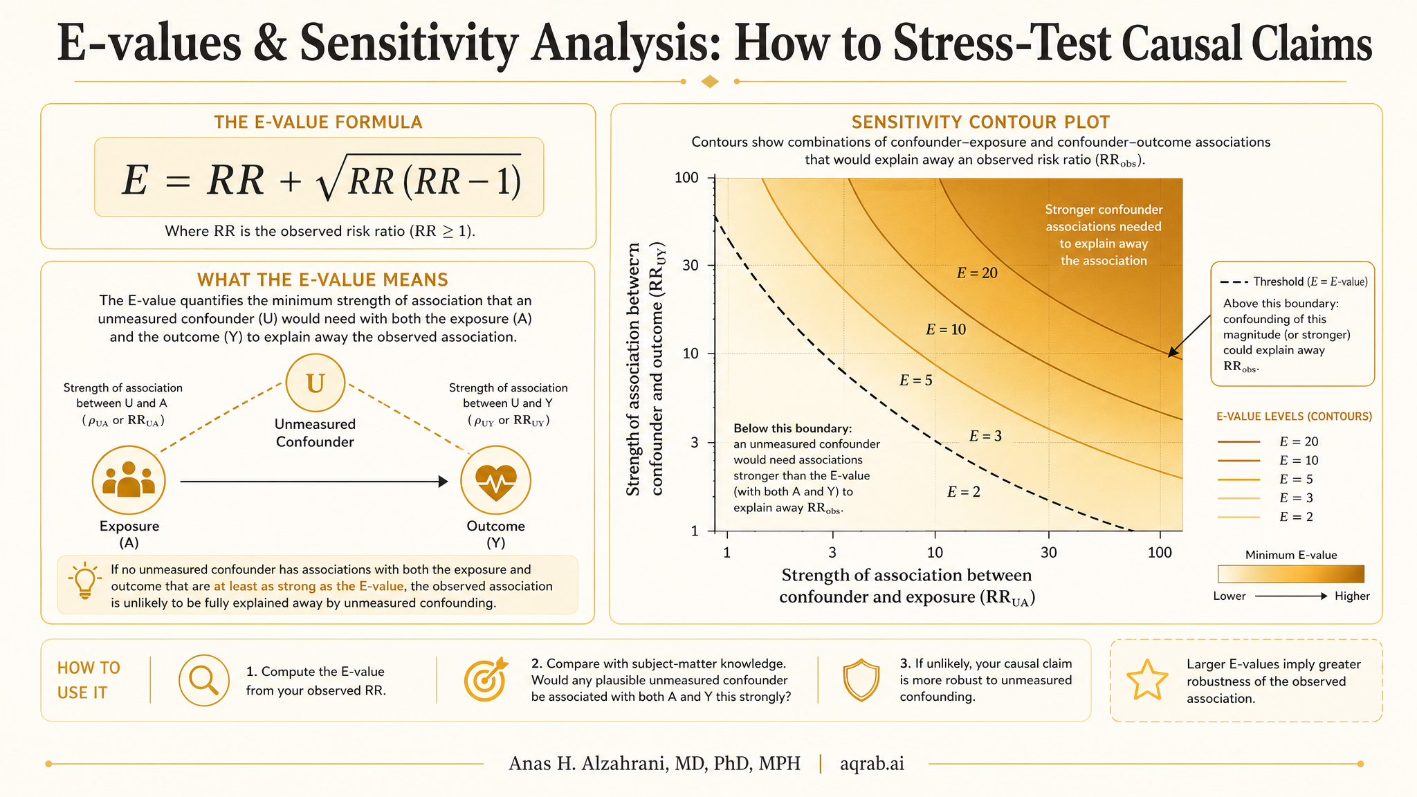
The E-value is a risk-ratio scale sensitivity metric. For a harmful or protective effect estimate, it asks: what is the minimum strength of association that a single unmeasured confounder would need with both the exposure and the outcome — conditional on the measured covariates — to explain away the observed association?
✓ What the E-value gives you
- A transparent benchmark for robustness to unmeasured confounding
- A number reviewers can compare with plausible real-world confounders
- A way to discuss uncertainty without pretending unmeasured confounding does not exist
✗ What the E-value does not give you
- Proof that your study is causal
- Protection against selection bias, measurement error, or immortal time bias
- Any insight about the direction or real-world existence of a confounder
- A replacement for domain knowledge or DAG-based reasoning
Big E-value, stronger claim. Small E-value, fragile claim. That is the basic intuition. If your observed risk ratio is 2.4 and the E-value is 4.2, then only a fairly strong unmeasured confounder could wipe it out. If your E-value is 1.4, the result is soft as hell — many ordinary omitted confounders could do that.
Practical rule
Never report only the E-value for the point estimate. Also report the E-value for the confidence interval limit closest to the null. That is the robustness of the inferential boundary — and usually the more honest number.
3. How to interpret E-values without lying to yourself
Here is the clean interpretation: an E-value of 2.8 means an unmeasured confounder would need to be associated with both exposure and outcome by a risk ratio of at least 2.8 each, above and beyond the measured covariates, to explain away the estimate.
But the number only means something relative to plausible omitted confounders. In some settings, an unmeasured factor associated with both treatment and outcome by a risk ratio of 2 is totally believable. In others, it is wildly implausible. That is why the best papers compare the E-value to known confounders in the literature, or at least discuss whether such a confounder could realistically exist.
4. Clinical example: statins and mortality
Suppose you study whether statin initiation after vascular surgery reduces one-year mortality using registry data. You adjust for age, sex, comorbidity burden, prior admissions, diabetes, renal disease, procedure type, and hospital. Your weighted analysis gives a hazard ratio of 0.72 for mortality.
Good. But now the real question: could the apparent benefit just reflect that the patients who got statins were also healthier, more adherent, or had better outpatient follow-up in ways your registry did not capture?
Measured covariates
- Age, sex, race/ethnicity
- Comorbidity index, CKD, diabetes
- Procedure type and urgency
- Hospital characteristics
- Prior admissions and medication burden
Likely unmeasured threats
- Frailty not captured administratively
- Functional status
- Medication adherence culture
- Physician preference
- Subtle disease severity markers
If the E-value for the point estimate is 2.1 and the E-value for the confidence limit is 1.6, the story becomes straightforward: the apparent benefit is not wildly robust. A moderately strong omitted confounder could still knock the result toward the null. That does not make the study useless. It means you should describe it as suggestive, not definitive.
The honest conclusion
“Our findings were moderately robust to unmeasured confounding, but an omitted factor associated with both statin initiation and mortality by a modest magnitude could attenuate the association.” That is a lot better than pretending the analysis proves causality.
5. When to use E-values — and when not to
Good use cases
- • Observational studies with a clear primary causal estimate
- • Cohort or case-control analyses after measured confounder adjustment
- • Papers where reviewers will rightly ask about residual confounding
- • Studies using PSM, IPW, outcome regression, or doubly robust estimators
- • Sensitivity appendices where you want one interpretable benchmark
Bad use cases
- • When the main design is broken by immortal time bias or selection bias
- • When positivity is awful and your effect estimate is already unstable
- • When exposure or outcome are badly misclassified
- • When you use E-values as the only sensitivity analysis
- • When the estimate is already near-null and clinically trivial
My view: E-values are best used as a minimum standard, not the whole show. If you are making a bold causal claim from nonrandomized data, a single scalar summary is not enough. Use it, but do not hide behind it.
6. Six ways sensitivity analysis gets abused
1. Using E-values to compensate for design errors
If your study has immortal time bias, collider stratification, or time zero misalignment, an E-value is lipstick on a structural flaw. It only addresses unmeasured confounding.
2. Reporting only the point-estimate E-value
That is the flattering number. The confidence-limit E-value is usually more conservative and more informative for inference.
3. Ignoring whether the confounder is plausible
An E-value of 2.3 sounds solid until you realize frailty or smoking severity could easily reach that scale in your dataset. Sensitivity metrics must be anchored to domain reality.
4. Treating hazard ratios, odds ratios, and risk ratios as interchangeable
E-values are defined on the risk-ratio scale. Approximation shortcuts exist, but careless conversion can make the sensitivity analysis look more robust than it really is.
5. Skipping sensitivity analysis because the p-value is small
A tiny p-value says nothing about omitted variable bias. Precision and validity are different problems.
6. Pretending one-number sensitivity analysis settles the question
It does not. Robust causal inference uses triangulation: design logic, negative controls, quantitative bias analysis, and sensitivity analyses that reflect the real data-generating threats.
7. Beyond E-values: stronger sensitivity analyses
If you want a paper that actually survives review, do more than calculate an E-value. Better options include:
Negative control outcomes or exposures
If your treatment “causes” something it biologically cannot cause, your residual bias is showing.
Quantitative bias analysis
Explicitly specify bias parameters for a hypothetical confounder and show how the estimate shifts across plausible ranges.
Rosenbaum bounds
Useful for matched studies when you want to ask how strong hidden bias would need to be to alter the inference.
Cinelli–Hazlett omitted variable bias analysis
Excellent for linear regression settings because it benchmarks omitted confounding against observed covariates.
The best workflow is simple: DAG first, primary estimate second, sensitivity analysis third, humility throughout. That order matters.
8. Reporting checklist for reviewers
If you include an E-value or any residual confounding analysis, reviewers should not have to guess what you did.
State the primary causal estimand clearly: ATE, ATT, risk ratio, hazard ratio, etc.
Explain which biases remain plausible after measured confounder adjustment and why unmeasured confounding is the focus.
Report the E-value for both the point estimate and the confidence interval limit closest to the null.
Specify any effect-scale approximation used if your main result was not naturally on the risk-ratio scale.
Compare the E-value with plausible real-world confounders from the literature or known clinical mechanisms.
Describe complementary sensitivity analyses, such as negative controls, Rosenbaum bounds, or quantitative bias analysis.
Do not overclaim. Use language like robust, moderately robust, or sensitive — not proof.
Clarify what the E-value does not address: measurement error, selection bias, missing data mechanisms, or time-zero problems.
9. Getting automated critique with Aqrab
Aqrab does not just ask whether your model converged. It asks the question reviewers actually care about: is the causal claim structurally defensible? That includes residual confounding, estimand mismatch, and whether your “robust” result is one omitted variable away from collapse.
Try Aqrab free
3 free critiques. No credit card. See whether your causal claim survives contact with reality.
Keep reading
Don't stop at one method.
Good methods judgment comes from contrast. Read the neighboring guides, see where the assumptions diverge, and avoid treating every observational problem like it needs the same hammer.
Proximal Causal Inference: What to Do When Unmeasured Confounding Is Still on the Table
A practical guide to proximal causal inference for clinical researchers. Covers proxy variables, treatment-inducing versus outcome-inducing proxies, bridge functions, completeness, and why this method is powerful but brutally assumption-heavy.
Instrumental Variables: When Observational Data Meets Unmeasured Confounding
When PSM and regression fail because of unmeasured confounding, IV methods offer a way forward. A practical guide covering instruments, LATE, Mendelian randomization, and the exclusion restriction.
Treatment-Induced Mediator-Outcome Confounding: When Mediation Analysis Starts Chasing the Consequences of Treatment
A practical guide to treatment-induced mediator-outcome confounding for clinical researchers. Covers why natural direct and indirect effects fail when treatment changes later severity, toxicity, adherence, or surveillance that affect both the mediator and outcome.
Further Reading
- VanderWeele TJ, Ding P. Sensitivity analysis in observational research: introducing the E-value. Annals of Internal Medicine. 2017;167(4):268-274.
- Mathur MB, VanderWeele TJ. Sensitivity analysis for unmeasured confounding in meta-analyses. Journal of the American Statistical Association. 2020;115(529):163-172.
- Cinelli C, Hazlett C. Making sense of sensitivity: extending omitted variable bias. Journal of the Royal Statistical Society Series B. 2020;82(1):39-67.
- Rosenbaum PR. Observational Studies. 2nd ed. Springer; 2002.
- Hernán MA, Robins JM. Causal Inference: What If. Chapman & Hall/CRC. 2020.