Causal Forests: Finding Treatment Effect Heterogeneity Without Fooling Yourself

1. Why average effects fail

Most causal inference papers report a single number: the average treatment effect. That is fine if your treatment effect is roughly constant. It is weak if treatment response varies meaningfully across age, baseline severity, genetics, comorbidity burden, adherence, or timing. The average can be positive even when the intervention is useless for half the population.

This is the clinical problem behind the hype around precision medicine. The real question is not just does treatment work? It is for whom, under what baseline profile, and by how much?Traditional subgroup analysis handles this badly. You pick a few cut points, run interaction terms, and hope the p-values behave. They usually don't.

Causal forests are one answer to that problem. Not magic. Not a free precision-medicine machine. But a disciplined way to estimate conditional average treatment effects while separating signal from overfit nonsense better than most ad hoc subgroup workflows.

2. What causal forests actually estimate

A causal forest estimates the treatment effect conditional on covariates:

The forest builds many trees, each splitting the data into subgroups where treatment effects appear more homogeneous within leaves and more different across leaves. But unlike ordinary prediction trees, the objective is not just predicting the outcome. The objective is learning how the difference between treated and untreated potential outcomes varies across covariate space.

This is the key thing people miss: causal forests are an estimation method, not an identification strategy. They sit downstream of your DAG, your confounder set, your overlap assumptions, and your study design. If the design is trash, the forest will estimate heterogeneity in trash.

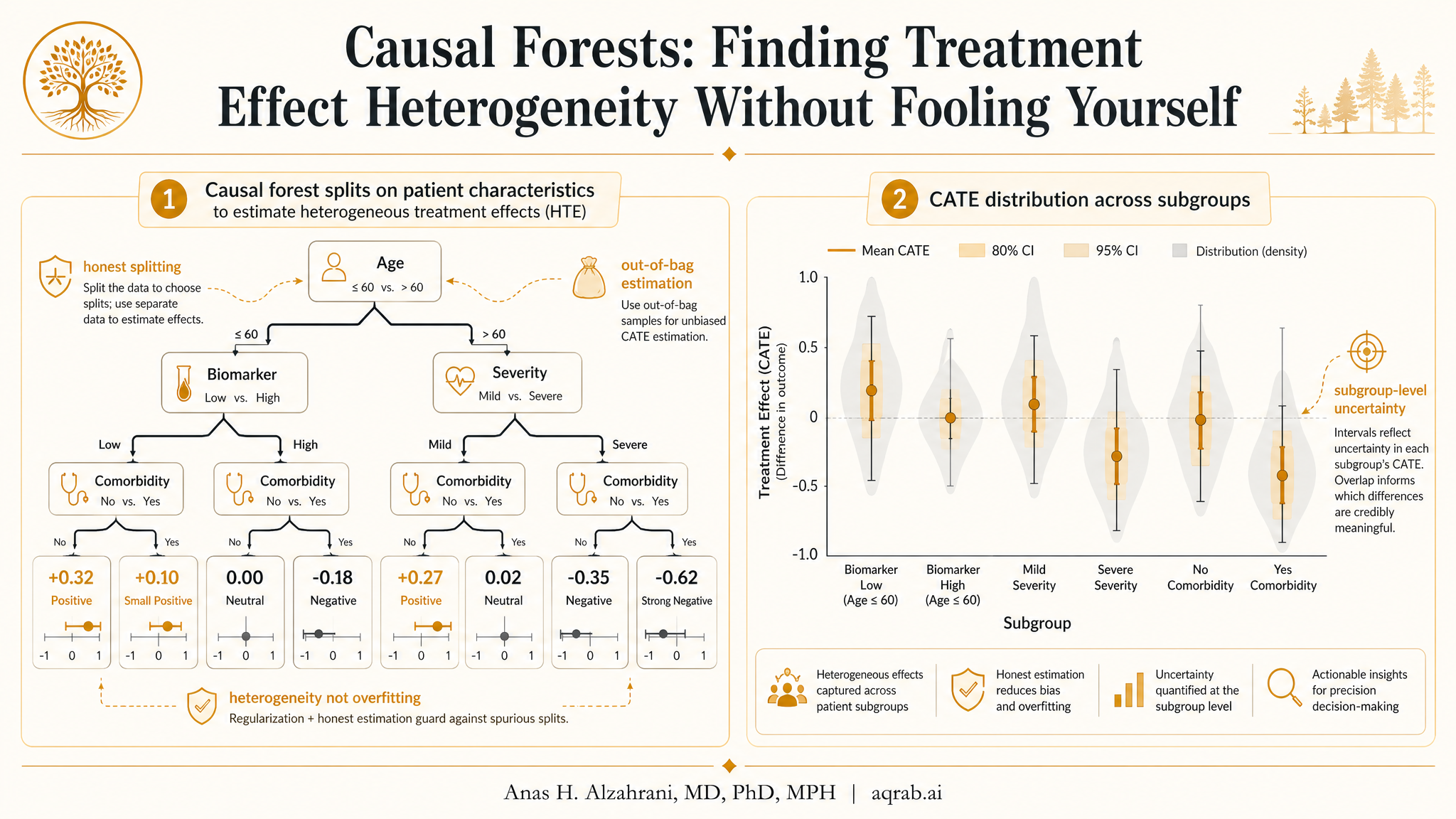
3. Honest splitting: the trick that makes them causal

Random forests are great at overfitting if you let them. The core innovation in causal forests, especially the generalized random forest framework from Athey, Tibshirani, and Wager, is honesty. The data used to choose splits are separated from the data used to estimate treatment effects within leaves.

That sounds like a technical detail. It isn't. Without honesty, the tree uses random noise twice — once to decide where the “interesting” subgroup is, and again to estimate the subgroup effect. That gives you exaggerated heterogeneity and fake confidence. Honesty reduces that bias.

4. When causal forests are worth using

Use causal forests when heterogeneity is central to the question, your sample is reasonably large, and you have credible covariate information measured before treatment. If all you want is the overall ATE, simpler estimators are easier to explain and often more efficient.

My blunt take: if your dataset has 300 patients and you want patient-level treatment recommendations, causal forests are probably bullshit. They need data density. Not infinite data, but enough information that local comparisons are meaningful.

5. Clinical example: who benefits from GLP-1 therapy?

Suppose you want to estimate which patients with obesity and type 2 diabetes derive the largest reduction in major adverse cardiovascular events from initiating a GLP-1 receptor agonist versus an alternative second-line agent.

A causal forest might show that younger low-risk patients have near-zero absolute benefit, while older patients with established ASCVD and high baseline risk have substantially larger predicted benefit. That is clinically useful — but only if you report uncertainty honestly and do not pretend the model found individualized truth for every patient.

6. How to interpret CATEs without lying to yourself

The most honest way to use causal forests is not to claim “this exact patient has a treatment effect of 3.7%.” That level of certainty is fake. A better workflow is:

In practice, causal forests are strongest as a ranking tool and a heterogeneity discovery tool. They are weaker as a basis for exact individualized treatment rules unless you have very strong validation. Distinguish exploratory heterogeneity from deployable treatment assignment.

7. Six failure modes that break most analyses

8. What reviewers should expect

If a paper uses causal forests and only reports a pretty heterogeneity plot, that is not enough. The reporting standard should be much higher.

One more thing: show the boring stuff. Reviewers should see overlap plots, event counts, and validation performance — not just an eye-catching tree diagram and a claim that machine learning found “hidden subgroups.”

9. Software and implementation

The most widely used implementation is the grf package in R. Python users often reach for EconML, which provides causal forest-style estimators and related learners. The right package matters less than whether you understand the estimand, overlap, and validation plan.

library(grf)

forest <- causal_forest(
  X = covariates,
  Y = outcome,
  W = treatment,
  num.trees = 2000,
  honesty = TRUE,
  tune.parameters = "all"
)

cate_hat <- predict(forest)$predictions
ate_hat <- average_treatment_effect(forest)

# Rank patients into quartiles of predicted benefit
quartile <- cut(cate_hat, quantile(cate_hat, probs = seq(0, 1, 0.25)), include.lowest = TRUE)
                

That code is the easy part. The hard part is whether your covariates are pre-treatment, whether your treatment definition avoids immortal time bias, whether overlap holds, and whether your heterogeneity ranking survives validation.

10. Getting automated critique with Aqrab

Aqrab is built for exactly this kind of methodological weak spot. If your study claims treatment effect heterogeneity, Aqrab checks whether the estimand is clear, whether the design actually supports causal interpretation, whether overlap is plausible, and whether your reporting is doing science or marketing.