G-Estimation: The Causal Method You Reach For When Time-Varying Confounding Breaks Regression
Most clinical researchers know three moves: regress on confounders, match on a propensity score, or weight the sample. All three start to wobble when treatment decisions evolve over time and the covariates driving those decisions are themselves changed by earlier treatment. That is where g-estimation enters. It is not the fashionable method. It is not the one most papers explain well. But in the right longitudinal setting, it is one of the cleanest ways to estimate a causal effect without conditioning away the very mechanism you care about.
In this guide
- 1. Why standard methods fail in longitudinal treatment decisions
- 2. What g-estimation is actually estimating
- 3. Structural nested models, without the unnecessary mysticism
- 4. Clinical example: dynamic treatment in HIV care
- 5. How g-estimation works step by step
- 6. Assumptions you cannot afford to wave away
- 7. G-estimation vs MSMs vs ordinary regression
- 8. Six ways published analyses quietly fail
- 9. What reviewers should expect in a serious paper
- 10. Using Aqrab to stress-test your design
1. Why standard methods fail in longitudinal treatment decisions
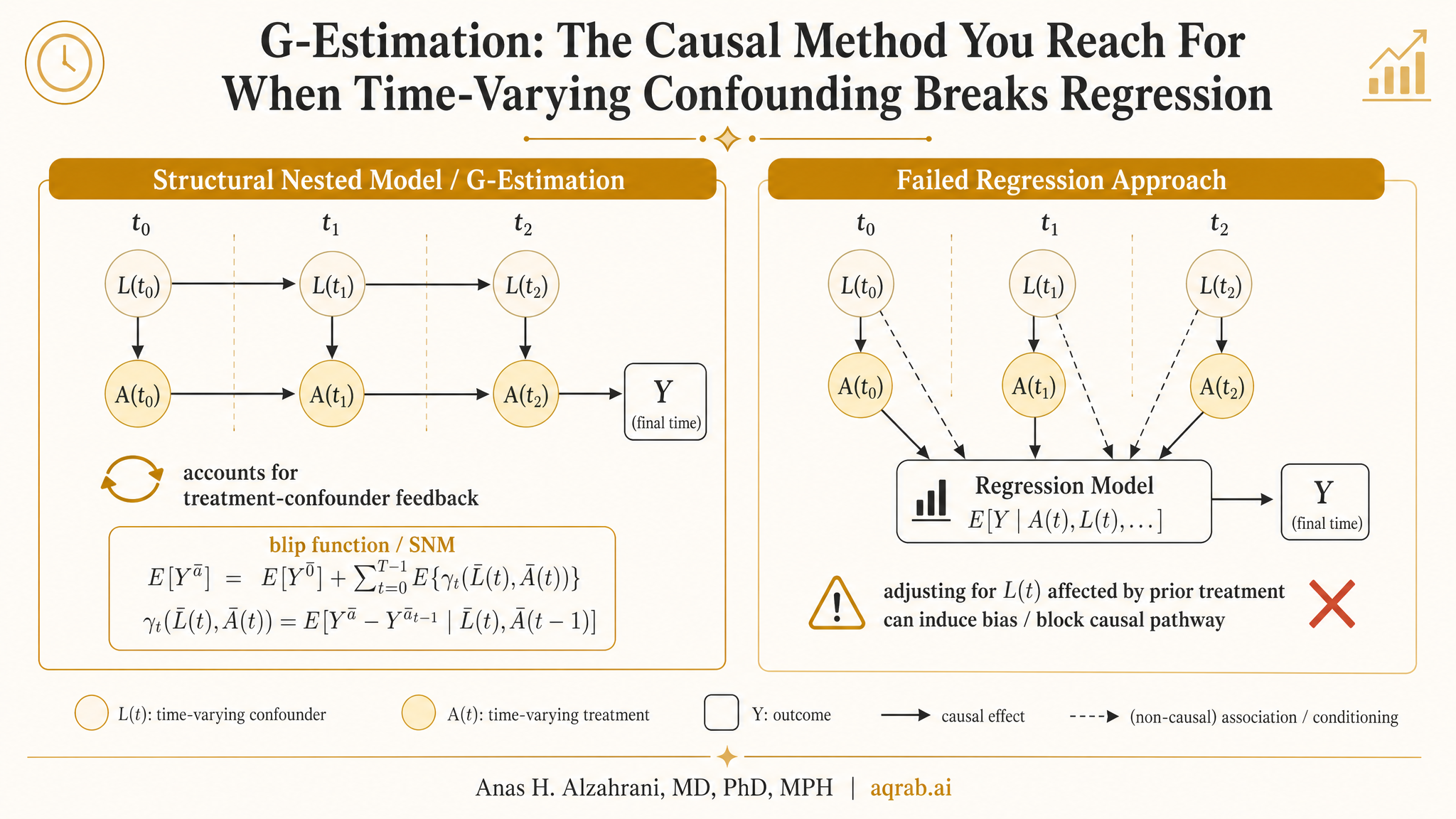
Imagine a chronic disease cohort where treatment is updated every few months. Physicians escalate, de-escalate, or stop therapy based on evolving biomarkers, symptoms, adverse effects, and prior response. Those evolving variables are confounders for the next treatment decision. But they are also downstream consequences of earlier treatment.
That creates the classic treatment-confounder feedback problem. If you adjust for the time-varying covariate with ordinary regression, you may control away part of the treatment effect. If you ignore it, you leave confounding behind. Standard regression is stuck in a lose-lose choice.
The core problem in one sentence
When a variable is both a confounder of future treatment and a consequence of past treatment, naive adjustment breaks causal interpretation.
This is why g-methods exist. Marginal structural models solve the problem by weighting. G-computation solves it by modeling counterfactual outcomes. G-estimation solves it by identifying the treatment effect that makes the residualized outcome independent of treatment, conditional on the right history. That sounds abstract. Keep going — the logic is cleaner than the jargon suggests.
2. What g-estimation is actually estimating
G-estimation is usually used with structural nested models (SNMs), especially structural nested mean models. The idea is to parameterize how treatment changes the outcome, then search for the treatment-effect parameter that removes any remaining association between treatment and the treatment-free potential outcome.
Translation into plain English
You guess a value for the causal effect, subtract that hypothesized treatment effect out of the observed outcome, and then ask: “If I got the effect right, would treatment still predict what remains?” If yes, your guess is wrong. If no, you found the parameter that makes treatment look conditionally randomized with respect to the blipped-down outcome.
That “blipped-down” language is old Robins terminology, and honestly it scares people off for no good reason. Think of it as removing the treatment effect from the outcome under a candidate parameter value, then checking whether the remaining outcome still helps explain treatment.
3. Structural nested models, without the unnecessary mysticism
Structural nested models describe how a treatment at a given time changes the potential outcome, given treatment and covariate history. Unlike MSMs, which target marginal effects under treatment regimes, SNMs are naturally framed around conditional causal contrasts over time.
Why people like SNMs
- • They handle time-varying confounding affected by prior treatment
- • They can target treatment effects conditional on history
- • They avoid building unstable inverse-probability weights
- • They can be more efficient when the treatment model is well specified
Why people avoid them
- • The notation looks like a dare
- • The intuition is rarely explained clearly
- • Software is less turnkey than basic regression or matching
- • Reviewers often know MSMs better, so papers oversell weights and ignore alternatives
My take: most researchers do not avoid g-estimation because it is weak. They avoid it because it is cognitively expensive, and because the average methods paper explains the algebra long before it explains the scientific use case.
4. Clinical example: dynamic treatment in HIV care
The canonical setting is HIV treatment, where therapy decisions evolve over follow-up based on CD4 count, viral load, toxicity, and adherence. CD4 count at month 6 affects the clinician's decision to continue or modify therapy, but that month-6 CD4 count was itself influenced by therapy before month 6.
Exposure
Start or intensify antiretroviral therapy at each visit.
Outcome
Progression to AIDS or death over follow-up.
Time-varying confounders
CD4 count, viral load, opportunistic infections, adverse effects, and adherence.
Why ordinary adjustment fails
Adjusting for current CD4 blocks part of the earlier treatment effect. Ignoring it leaves confounding in later treatment choices.
A structural nested mean model can parameterize how treatment at each visit shifts the expected counterfactual outcome. G-estimation then finds the effect size that makes the adjusted treatment-free outcome no longer predict subsequent treatment, given observed history. In other words: after removing the candidate treatment effect, the remaining variation should not tell you who got treated, if the causal parameter is correct.
5. How g-estimation works step by step
Specify the causal model
Write down a structural nested model for how treatment at time t changes the outcome, conditional on history. This is the scientific backbone, not just a technical convenience.
Choose a candidate treatment effect
Pick a value for the causal parameter. Think of it as your current guess for how much treatment changes the outcome.
Blip down the outcome
Subtract the hypothesized treatment effect from the observed outcome to create the treatment-free or residualized outcome under that candidate parameter.
Fit the treatment model
Model treatment as a function of measured history and the blipped-down outcome. If the guessed effect is wrong, the blipped-down outcome will still help predict treatment.
Search for the parameter that kills that association
The g-estimate is the value at which the residualized outcome no longer predicts treatment after conditioning on observed history.
Estimate uncertainty correctly
Use appropriate variance estimation, bootstrap procedures, or estimating-equation methods. If your inferential step is hand-wavy, the whole thing becomes a math cosplay exercise.
The logic is elegant: a correct treatment-effect parameter makes the treatment-free potential outcome conditionally independent of treatment assignment. That is the estimating principle. Everything else is implementation detail.
6. Assumptions you cannot afford to wave away
No unmeasured confounding, sequentially
At each treatment time, after conditioning on measured history, treatment assignment should not depend on future counterfactual outcomes. This is the same core exchangeability assumption you need for MSMs, but applied in a structural nested framework.
Consistency
The observed outcome under the observed treatment history equals the potential outcome under that same treatment history. If treatment is vaguely defined, or adherence makes “treatment” slippery, consistency becomes fragile fast.
Positivity
Every relevant treatment option must remain possible within levels of observed history. If a subgroup is always treated or never treated, the data do not identify the counterfactual contrast there.
Correct model specification
G-estimation lives and dies on the models you specify: the structural nested model and the treatment model. If the functional form is badly wrong, the estimating equation can point confidently in the wrong direction.
None of these assumptions are decorative. If your paper uses the phrase “we applied g-estimation to control for time-varying confounding” without showing why those assumptions are plausible, it is not rigorous — it is incantation.
7. G-estimation vs MSMs vs ordinary regression
If you need a marginal population-level effect under time-varying treatment, MSMs are often easier to communicate. If your weights explode or your scientific question is naturally framed through conditional treatment effects over history, g-estimation deserves a serious look. It is not “better” in every case. It is often better aligned with the problem.
8. Six ways published analyses quietly fail
1. Treating g-estimation like a black-box sensitivity analysis
It is not a magic robustness button. It is a model-based causal estimator with hard assumptions.
2. Including post-treatment variables in the wrong part of the model
Temporal ordering matters. Sloppy history definitions turn causal modeling into a time-travel bug.
3. Using vague treatment definitions
If “treated” mixes initiation, switching, dose intensity, and adherence, consistency becomes fiction.
4. Ignoring positivity problems because the treatment model converged
Numerical convergence is not evidence of identification. Deterministic treatment patterns still wreck causal interpretation.
5. Reporting only point estimates with no explanation of the estimating strategy
If a reader cannot reconstruct how the parameter was found, the methods section failed.
6. Comparing g-estimation to naive regression and declaring victory without triangulation
A better workflow is to triangulate across g-methods and explain why estimates agree or diverge.
9. What reviewers should expect in a serious paper
A clear causal question and explicit treatment regime or decision process
A timeline showing when covariates, treatment decisions, censoring, and outcomes occur
A structural nested model written in interpretable form, not buried in supplemental algebra only
A transparent description of the treatment model used in the estimating step
Why treatment-confounder feedback exists and why ordinary adjustment would be biased
Evidence that positivity is plausible in the observed data
How uncertainty was estimated: bootstrap, sandwich estimator, or estimating equations
Sensitivity analyses or triangulation against MSMs, g-computation, or clinically motivated alternatives
A plain-language interpretation of the parameter for clinicians and reviewers
Limitations that explicitly address unmeasured confounding and model misspecification
Reviewers are usually much more forgiving of mathematical complexity than conceptual vagueness. If you show the timeline, the causal problem, and the estimating logic clearly, g-estimation becomes defensible. If you hide behind notation, the paper will look like a bluff.
10. Using Aqrab to stress-test your design
Aqrab is built for exactly this sort of methods choice. If you are deciding between longitudinal regression, MSMs, g-estimation, or g-computation, the platform can critique the causal structure, flag treatment-confounder feedback, and tell you whether your estimand matches your data and timeline. That matters more than picking the method with the coolest name.
Try Aqrab free
Paste your protocol, methods, or DAG and get a structured critique before a reviewer tears it apart.
Keep reading
Don't stop at one method.
Good methods judgment comes from contrast. Read the neighboring guides, see where the assumptions diverge, and avoid treating every observational problem like it needs the same hammer.
Time-Varying Confounding: When Yesterday's Treatment Changes Today's Confounder
A practical guide to time-varying confounding for clinical researchers. Covers treatment-confounder feedback, why ordinary regression fails, and how MSMs, g-methods, and target trial logic handle evolving treatment decisions.
Parametric G-Formula: Estimating Causal Effects When Covariates Change Over Time
A practical guide to the parametric g-formula for clinical researchers. Covers time-varying confounding, dynamic treatment strategies, longitudinal simulation, model diagnostics, and why ordinary regression breaks when covariates are changed by prior treatment.
Treatment-Induced Mediator-Outcome Confounding: When Mediation Analysis Starts Chasing the Consequences of Treatment
A practical guide to treatment-induced mediator-outcome confounding for clinical researchers. Covers why natural direct and indirect effects fail when treatment changes later severity, toxicity, adherence, or surveillance that affect both the mediator and outcome.
Further Reading
- Robins JM. A new approach to causal inference in mortality studies with sustained exposure periods — application to control of the healthy worker survivor effect. Mathematical Modelling. 1986;7(9-12):1393-1512.
- Robins JM, Hernán MA, Brumback B. Marginal structural models and causal inference in epidemiology. Epidemiology. 2000;11(5):550-560.
- Hernán MA, Robins JM. Causal Inference: What If. Chapman & Hall/CRC. 2020.
- Daniel RM, De Stavola BL, Cousens SN. gmethods, structural nested models and the g-formula: a commentary on causal inference in longitudinal studies. Statistical Methods in Medical Research. 2011;20(6):597-619.
- Vansteelandt S, Joffe M. Structural nested models and g-estimation: the partially realized promise. Statistical Science. 2014;29(4):707-731.
- Keil AP, Edwards JK, Richardson DB, Naimi AI, Cole SR. The parametric g-formula for time-to-event data: towards intuition with a worked example. Epidemiology. 2014;25(6):889-897.